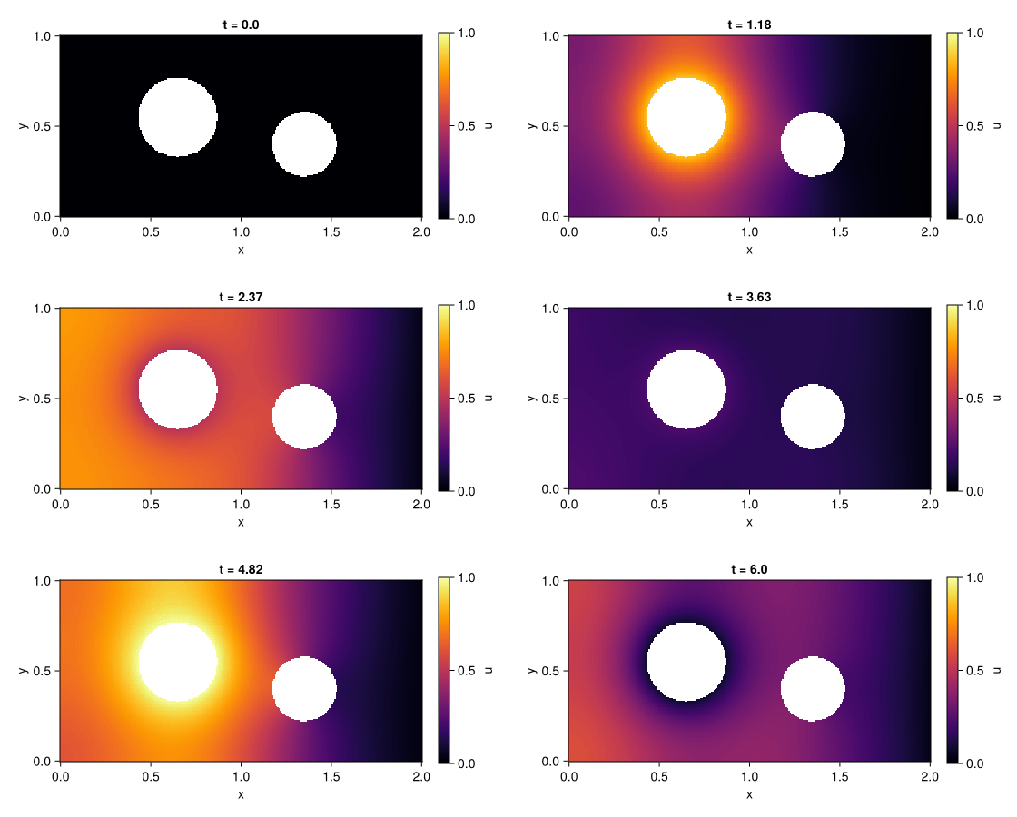
FiniteElementMethod.jl

FiniteElementMethod.jl solves PDEs written in strong form with ModelingToolkit.jl on unstructured meshes. Write the equation and its boundary conditions as you would on paper, put them on a Gmsh geometry, and the package derives the Galerkin weak form, assembles it with Ferrite.jl and hands you a DAEProblem for the DifferentialEquations.jl solvers. No mesh loops, no weak forms by hand, and no scalarisation: each field is one array unknown.

The animation above is this code, run by the documentation build:

using FiniteElementMethod, ModelingToolkit, DomainSets, FerriteGmsh, OrdinaryDiffEqBDF
using ModelingToolkit: t_nounits as t

@parameters k α
@variables x y u(..)
Dt, Dx, Dy = Differential(t), Differential(x), Differential(y)

grid = togrid(pkgdir(FiniteElementMethod, "examples", "plate.geo"))   # Gmsh physical groups become pieces
Ω = MeshDomain(grid)
Γ_in, Γ_wall, Γ_out = boundarypiece.(Ω, (:inlet, :wall, :outlet))
Dn_wall, Dn_out = NormalDerivative(Γ_wall), NormalDerivative(Γ_out)

eqs = [Dt(u(t, x, y)) ~ Dx(k * Dx(u(t, x, y))) + Dy(k * Dy(u(t, x, y)))]
bcs = [
    u(t, Γ_in) ~ sin(t)^2,                          # Dirichlet: a pulsing heated pipe
    Dn_wall(u(t, Γ_wall)) ~ 0,                      # Neumann: insulated edges and second hole
    k * Dn_out(u(t, Γ_out)) + α * u(t, Γ_out) ~ 0,  # Robin: convective cooling
    u(0, x, y) ~ 0,
]
domains = [(x, y) ∈ Ω, t ∈ Interval(0.0, 6.0)]
@named pdesys = PDESystem(eqs, bcs, domains, [t, x, y], [u(t, x, y)], [k => 0.2, α => 2.0])

sol = solve(discretize(pdesys, FEMDiscretization(Ω, t)), DFBDF())
sol(6.0, 1.0, 0.9; dv = u(t, x, y))                 # the temperature at any point, at any time

x and y are bound to the mesh by (x, y) ∈ Ω, conditions live on named boundary pieces as traces u(t, Γ) and normal derivatives NormalDerivative(Γ), and the solution is indexed and called in the same symbols. The documentation covers how this differs from MethodOfLines.jl.

A boundary with no condition gets the natural zero-flux condition, with a warning that lists it; declare it with FEMDiscretization(Ω, t; natural = [Γ_out]), or make the warning an error with boundary_check = :error. A boundary given as a lower-dimensional mesh becomes a piece with add_boundary_pieces!(grid, :inlet => inlet_mesh). See boundary conditions.

Navier–Stokes

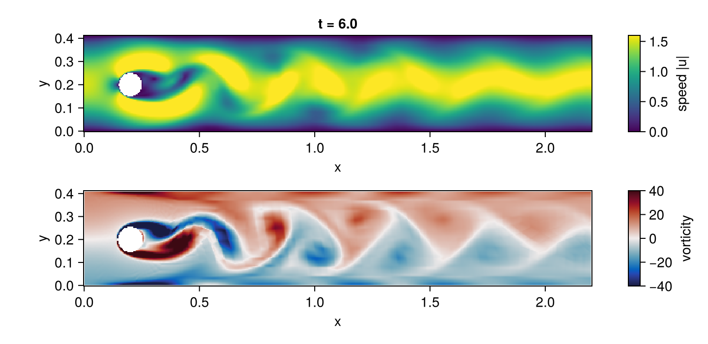
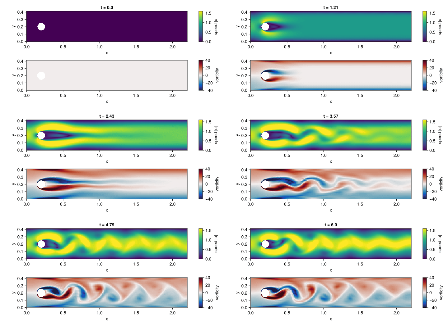
The incompressible Navier–Stokes equations are one more strong-form PDESystem: three equations for the velocity components u, v and the pressure p, discretized with Q2/Q1 Taylor–Hood elements and integrated as an index-2 DAE. The flow starts at rest in the DFG benchmark channel with a cylinder, at Reynolds number 100 (the inflow of case 2D-2), and sheds a vortex street. The images above are rendered by the two code blocks below, which examples/ns_showcase.jl runs as written (a test fails when they change without the images being regenerated). It is a showcase on a coarse mesh: the measured Strouhal number is about 0.3, the benchmark's value, but the run is not validated against the benchmark's shedding data. The steady Reynolds number 20 case (2D-1) is the one checked against its drag, lift and pressure difference.

using FiniteElementMethod, ModelingToolkit, DomainSets, OrdinaryDiffEqBDF
using OrdinaryDiffEqBDF: NLNewton
using LinearSolve: UMFPACKFactorization
using SciMLBase: CheckInit
using ModelingToolkit: t_nounits as t

include(pkgdir(FiniteElementMethod, "examples", "dfg_cylinder", "mesh.jl"))   # dfg_channel_grid: Gmsh quadrilaterals, curved cylinder

@parameters ν Umax
@variables x y u(..) v(..) p(..)
Dt, Dx, Dy = Differential(t), Differential(x), Differential(y)

Ω = MeshDomain(dfg_channel_grid(; h = 0.04, hc = 0.0025))
Γ_in, Γ_out, Γ_wall, Γ_cyl = boundarypiece.(Ω, (:inlet, :outlet, :walls, :cylinder))
U, V, P = u(t, x, y), v(t, x, y), p(t, x, y)

eqs = [
    Dt(U) ~ Dx(ν * Dx(U)) + Dy(ν * Dy(U)) - U * Dx(U) - V * Dy(U) - Dx(P),
    Dt(V) ~ Dx(ν * Dx(V)) + Dy(ν * Dy(V)) - U * Dx(V) - V * Dy(V) - Dy(P),
    0 ~ Dx(U) + Dy(V),                                       # incompressibility: no equation for p
]
inflow = (1 - exp(-t^2)) * 4Umax * y * (0.41 - y) / 0.41^2   # parabolic, ramped up from rest
bcs = [
    u(t, Γ_in) ~ inflow, v(t, Γ_in) ~ 0,
    u(t, Γ_wall) ~ 0, v(t, Γ_wall) ~ 0,
    u(t, Γ_cyl) ~ 0, v(t, Γ_cyl) ~ 0,                        # no slip
    p(t, Γ_out) ~ 0,                                         # fixes the pressure level at the outlet
    u(0, x, y) ~ 0, v(0, x, y) ~ 0,
]
tend = 6.0
domains = [(x, y) ∈ Ω, t ∈ Interval(0.0, tend)]
@named dfg = PDESystem(eqs, bcs, domains, [t, x, y], [U, V, P], [ν => 1.0e-3, Umax => 1.5])

Q2, Q1 = Lagrange{RefQuadrilateral, 2}(), Lagrange{RefQuadrilateral, 1}()
disc = FEMDiscretization(
    Ω, t; spaces = Dict(u => Q2, v => Q2, p => Q1),
    pairing = Dict(eqs[3] => p), natural = [Γ_out], initializealg = CheckInit()
)
prob = discretize(dfg, disc)
abstol = [differential ? 1.0e-6 : 1.0e8 for differential in prob.differential_vars]   # no error control on p
sol = solve(prob, DFBDF(nlsolve = NLNewton(new_W_dt_cutoff = 0), linsolve = UMFPACKFactorization()); abstol, reltol = 1.0e-6)
sol(tend, 0.6, 0.2; dv = v(t, x, y))                         # the cross-stream velocity in the wake

The solution is then resampled on a regular grid with sol(ts, xs, ys; dv), which returns NaN inside the cylinder, and plotted with Makie. CairoMakie is not a dependency of FiniteElementMethod: install it with using Pkg; Pkg.add("CairoMakie"), then run this block in the same session as the block above, in the directory that should receive the two images.

using CairoMakie

xs, ys = range(0, 2.2; length = 440), range(0, 0.41; length = 82)   # a regular grid over the channel
ts = range(0, tend; length = 90)
u_field = sol(collect(ts), collect(xs), collect(ys); dv = u(t, x, y))   # time × nx × ny
v_field = sol(collect(ts), collect(xs), collect(ys); dv = v(t, x, y))
speed = hypot.(u_field, v_field)
vorticity = fill(NaN, size(u_field))                                    # ∂ₓv − ∂ᵧu, central differences
i, j = 2:(length(xs) - 1), 2:(length(ys) - 1)
@views vorticity[:, i, j] .= (v_field[:, i .+ 1, j] .- v_field[:, i .- 1, j]) ./ 2step(xs) .-
    (u_field[:, i, j .+ 1] .- u_field[:, i, j .- 1]) ./ 2step(ys)

frame = Observable(length(ts))
fig = Figure(size = (720, 350))
axis_options = (; aspect = DataAspect(), xlabel = "x", ylabel = "y")
top = Axis(fig[1, 1]; title = @lift("t = $(round(ts[$frame]; digits = 2))"), axis_options...)
bottom = Axis(fig[2, 1]; axis_options...)
speed_map = heatmap!(top, xs, ys, @lift(speed[$frame, :, :]); colormap = :viridis, colorrange = (0, 1.6), nan_color = :white)
vorticity_map = heatmap!(bottom, xs, ys, @lift(vorticity[$frame, :, :]); colormap = :balance, colorrange = (-40, 40), nan_color = :white)
Colorbar(fig[1, 2], speed_map; label = "speed |u|")
Colorbar(fig[2, 2], vorticity_map; label = "vorticity")

save("ns_showcase.png", fig; px_per_unit = 2)                           # the flow at the final time
record(fig, "ns_showcase.gif", eachindex(ts); framerate = 18, px_per_unit = 1) do index
    frame[] = index
end

Benchmarks

Accuracy per degree of freedom against MethodOfLines, assembly cost against hand-written Ferrite, and problem construction time are regenerated by the documentation build, with the hardware, package versions and date of each run: see the benchmarks page.

What it solves

Second-order parabolic and elliptic equations, scalar or coupled multi-field, in divergence or non-divergence form, with nonlinear coefficients and sources, moderate convection, and Dirichlet, Neumann and Robin conditions, in 1D and 2D. The supported equation classes page lists every class with the evidence behind it, what is accepted but not yet reliable, and what is rejected with a clear error.